Lab 8, Modeling at Summit Gear: Specify, Fit, Interpret
You fit two models on one customer table this week, an OLS regression that forecasts how long an account takes to pay and a logistic regression that estimates whether a receivable goes bad. The AI writes the fitting code. Your graded work is the part it cannot do for you: specify the model, validate the fit, and interpret every number in collections terms.
The story of this lab, start here
You are an analyst at Summit Gear Co., a B2B outdoor-equipment wholesaler. The company sells on credit, so every new account is a small bet: the customer takes the goods now and pays the invoice later, and some never pay at all. The collections team lives with two questions on every account, and both are questions a model can answer. First, a number: how long will this account take to pay (days_to_pay), so the team knows when to expect the cash and when to start chasing it? Second, a yes/no: will this receivable default (defaulted), so the team knows which accounts to watch before the loss happens? They hand you one table, one row per customer, and ask you to answer both.
Those two questions need two different models. "How many days" is a number on a continuous scale, a forecasting problem, and calls for OLS regression. "Will it default" is a yes/no, a classification problem, and calls for logistic regression. This week you fit both, on the same customers, and part of the skill is learning to tell from the question alone which model it needs. The content below walks you through solving it, one exercise at a time.
The shift this week is where your work lives. In Week 7 you wrote the code. This week the AI writes the model-fitting code, and your job is the part the AI cannot do for you: specify the model (pick the target and the predictors, avoid look-ahead bias), validate that it ran cleanly and the predictors are sound, and interpret every number in collections terms. The AI fits; you decide what to fit and what the fit means.
What you'll do
Four exercises, all built on the one customer table: fit an OLS model for days_to_pay, clean it up with feature selection, fit a logistic model for defaulted, then have an AI turn your results into an explainer you assess. Each exercise below opens with a one-line "what to do here" so you always know the goal before you read the detail.
File -> Download -> Download .ipynb). Then, in the Lab 8 New Quiz, upload that notebook, generate and upload the HTML explainer (the full prompt is in the quiz), and answer the assessment question. That is the whole handoff, three modeling exercises here, the explainer and assessment in the quiz.
credit_limit, avg_balance, prior_late_count, days_since_last_order, and so on) is a customer attribute known at decision time, and neither target is computed from the other, so there is no leak to find here. The point is the habit: before you hand a column to a model, ask whether you would actually have it when the prediction is made.Get set up
The data. One row per Summit Gear B2B customer, 2,200 rows. The data dictionary names every column, its units, and which columns move together, read it before you specify a model. pandas is the default path here: the template notebook already points pd.read_csv() at the raw CSV URL, so you are loaded the moment it opens.
- CSVsummit_gear_customers.csv, the 2,200-row dataset, downloads on click. View / raw URL for pandas.
- MDsummit_gear_customers_dictionary.md, every column explained, downloads on click. View on GitHub.
- SQLitesummit_gear_customers.sqlite, the identical table as a SQLite database, downloads on click, if you would rather work in SQL.
Prefer SQL? The SQLite file holds the same rows as the CSV. You can query it right inside your notebook (sqlite3 plus pandas.read_sql) or open it in an in-browser SQL tool if you prefer, then pull the result into a DataFrame and the rest of the lab is unchanged. Pandas on the CSV stays the default path; SQL is there only if it fits how you work.
The notebook. There is one working notebook, the template, with all four exercises stubbed out and a testing function at the end. That is where your graded work happens. Open it in Colab to work in the browser, or download it and run it locally, same file either way.
- COLABOpen lab_08_template.ipynb in Google Colab, work it in the browser, no install
- IPYNBDownload lab_08_template.ipynb, to run locally
Tools. The notebook runs in Google Colab in your browser (no install) or any local Python with pandas, numpy, statsmodels, and scikit-learn. Every fitting step uses an AI assistant, either the tutor on this page or the one in your notebook environment (see the next section), which writes the fit lines for you. An optional Excel path for the OLS half is in the Build the OLS in Excel section after Exercise 2.
How to work this lab, the AI-first contract
You lean on an AI assistant for every fitting step, so first pick where that assistant lives. Two paths, take whichever fits your setup:
- Path A, Colab plus Gemini (the default). Open the template in Google Colab (the link above) and use Colab's built-in Gemini to write the fit lines right beside your cells, nothing to install. For questions about the lab itself rather than the code, the Ask-AI tutor on this page is set to the class Gemini tier for stronger answers, reach for it on "what does this coefficient mean" or "why drop this predictor."
- Path B, local notebook plus Claude. If you use Claude, download the template (the link above), add the Claude extension to your editor, and work the notebook locally. Same notebook, same exercises, same grading, just on your own machine.
Whichever path you pick, the working pattern is identical in all four exercises:
- You specify. Write, in plain words, the target and the predictor set you want, and why each predictor belongs. This is your input to the AI.
- The AI writes the code. Ask it for the
pandas/statsmodels/scikit-learnlines that fit exactly that model and print the output. Fitting a named model is precisely what AI is good at. - You validate and interpret. Run the code. Confirm it ran on the right rows with the right predictors. Then read every number back in collections terms, in your own words. That reading is the work that earns the judgment points.
The AI will write a fit line on request. It will not write your interpretation paragraph or your explainer assessment for you, if your answer box is empty it asks you to take a first pass first. That is the rule, not a bug: the interpretation is the graded work.
Exercise 1, Fit OLS for days_to_pay and interpret the coefficients 25 pts
What to do here: specify an OLS model for days_to_pay, have the AI fit it, and read the coefficient table in collections terms.
The question: how long does a customer take to pay, and what drives it?
Specify. The target is days_to_pay. For this first fit, use this predictor set (you will revise it in Exercise 2):
credit_limit, avg_balance, annual_spend, prior_late_count, days_since_last_order, orders_per_year, discount_rate, avg_order_value, noise_a, noise_b.
This is the "kitchen sink" model, every numeric predictor in the table. Fitting it first, on purpose, sets up the problem you solve in Exercise 2.
Let AI write the fit. Ask the tutor for the statsmodels OLS that regresses days_to_pay on those predictors and prints the coefficient table plus R² and adjusted R². Run it. Save the output in the cell.
statsmodels for OLS: import statsmodels.api as sm, then sm.OLS(y, sm.add_constant(X)).fit(), where y is the days_to_pay column and X is the predictor columns. sm.add_constant is what gives you the intercept term (the const row). Call .summary() on the fitted result for the coefficient table, R², and adjusted R².Validate. Confirm the model fit on all 2,200 rows and used the predictors you named. Read off the R² and adjusted R².
Interpret (this is the graded part). Write a short paragraph that answers:
- Read two coefficients in collections terms, in the form "holding the other predictors fixed, a one-unit increase in X changes predicted
days_to_payby b days." Pickprior_late_countand one other. - State what the R² says about how much of the in-sample variation in payment timing the model explains, in plain words. (These are illustrative in-sample numbers, not a claim about new customers.)
- Name one coefficient whose sign or size looks wrong or unstable and say you will come back to it. (You will: it is the collinearity problem.)
Write the helper. Fill in predicted_days:
def predicted_days(coefs, row):
    """TODO: one sentence, what does this return?"""
    return None
coefs is a dict of predictor name to coefficient (including the key const for the intercept). row is a dict of predictor name to value. Return the predicted days_to_pay for that customer: the intercept plus the sum of each coefficient times its value. This is "score one customer from a fitted model", the same arithmetic the AI's .predict() does, written once by hand so you know what it is doing.
predicted_days is auto-checked with held-out inputs and your fitted R² is checked against the key (~0.84), so keep the signature and the docstring; the interpretation paragraph is read against the rubric.Exercise 2, Feature selection: spot and drop a collinear predictor 25 pts
What to do here: use a correlation matrix to find predictors that move together, drop the redundant ones, and re-fit a cleaner OLS.
pandas and numpy; the fits across the lab also use statsmodels and scikit-learn. In Colab these come preinstalled. Working locally, install them once with pip install pandas numpy statsmodels scikit-learn. Build the correlation matrix with df[predictors].corr().The problem you set up in Exercise 1. Look at the kitchen-sink coefficient table. Three predictors, credit_limit, avg_balance, annual_spend, describe the same thing (a customer's account size) in three units. When predictors move together like that, the model cannot tell their effects apart, so their individual coefficients become unstable: inflated standard errors, and sometimes a sign that makes no business sense. This is multicollinearity, and diagnosing it is the most important judgment in this lab.
Diagnose with a correlation matrix. Ask the AI for a correlation matrix of the numeric predictors (the full set, or just the suspects). Read the off-diagonal cells: a cell close to 1.0 (or -1.0) between two different predictors is the warning sign that they move together. You will see credit_limit, avg_balance, and annual_spend all correlate above 0.96 with each other, three measures of one underlying thing, account size. The noise_a and noise_b columns correlate with nothing; they are not collinear, they are just useless, which is a different problem you also fix.
Write the helper. Fill in flag_collinear_pairs. It takes the correlation matrix itself, the same one you just built:
def flag_collinear_pairs(corr, threshold=0.9):
    """TODO: one sentence, what does this return?"""
    return None
What it takes: corr is the correlation DataFrame from df[predictors].corr(), a square table of pairwise correlations. What it returns: a list of (col_a, col_b, r) triples. Walk the upper triangle only (each pair once, skip the diagonal), and for every pair whose absolute correlation clears the bar (abs(r) >= threshold), append (col_a, col_b, r), where col_a and col_b are the two column names and r is their correlation. Use abs(...) so a strong negative correlation is caught too. That specific shape, a list of name-name-value triples, is what the auto-check and the final_check testing function expect, so return exactly that.
Decide and re-fit. Reduce the collinear cluster to one representative predictor and drop the noise columns. Ask the AI to re-fit the OLS on your reduced set and print the new coefficient table, R², and adjusted R².
Justify (this is the graded part). Write a short paragraph that answers:
- Which predictors were collinear, and what in the correlation matrix told you (name the hot cells)?
- Which one did you keep, and why one is enough.
- What happened to adjusted R² when you dropped the redundant and noise columns, and why dropping them was the right call even though plain R² barely moved. (More predictors is not a better model. Adjusted R² is the number that stops rewarding clutter.)
flag_collinear_pairs is auto-checked with held-out inputs and your reduced-model adjusted R² is checked against the key (~0.843), so keep the signature and the return shape; the feature-selection justification is read against the rubric. Run final_check() at the end of the notebook to confirm this helper passes before you submit.Click here to see it done in Excel
This section is optional and ungraded. The lab is Python-primary; this is a fast secondary path if you want to see the same days_to_pay fit built in a tool you already know. OLS runs in Excel through the Analysis ToolPak, and the correlation check from Exercise 2 runs there too. (Logistic regression in Excel is painful, so the logistic half of the lab stays in Python.)
The workbook is already loaded for you. Download the pre-built workbook, it has a Read me tab and a Data tab with all 2,200 customer rows already in place, so it is ready to complete with no import step.
- XLSXsummit_gear_customers.xlsx, pre-loaded workbook, Read me + Data tabs, downloads on click. View on GitHub.
Turn on the Analysis ToolPak (one time)
It ships with Excel but is off by default: File -> Options -> Add-ins -> Manage: Excel Add-ins -> Go -> check Analysis ToolPak -> OK. A Data Analysis button then appears at the right end of the Data tab.
Run the regression
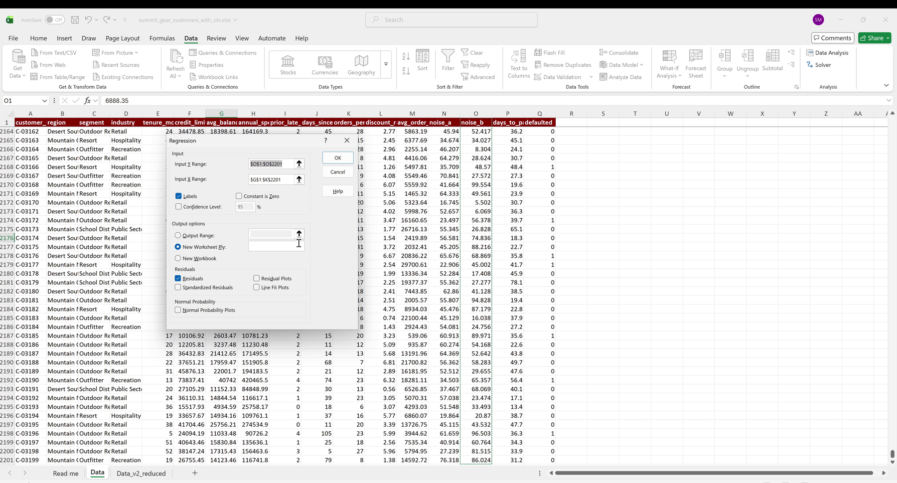
On the Data tab, click Data Analysis -> Regression, then fill the dialog:
- Input Y Range: the
days_to_paycolumn (your model's target), including its header. - Input X Range: the numeric predictor columns. For your first run use all of them, columns E through O (
tenure_monthsthroughnoise_b); they are already contiguous. (If you ever want a custom subset, arrange those columns adjacent first.) - Check Labels (since you included the header row), and choose an output location.
Read the output
Excel prints a summary block. The pieces that match the Python output: R Square (the same R² you read in Exercise 1), and the Coefficients column in the lower table (the intercept plus one row per predictor, the same coefficients you interpret in collections terms).
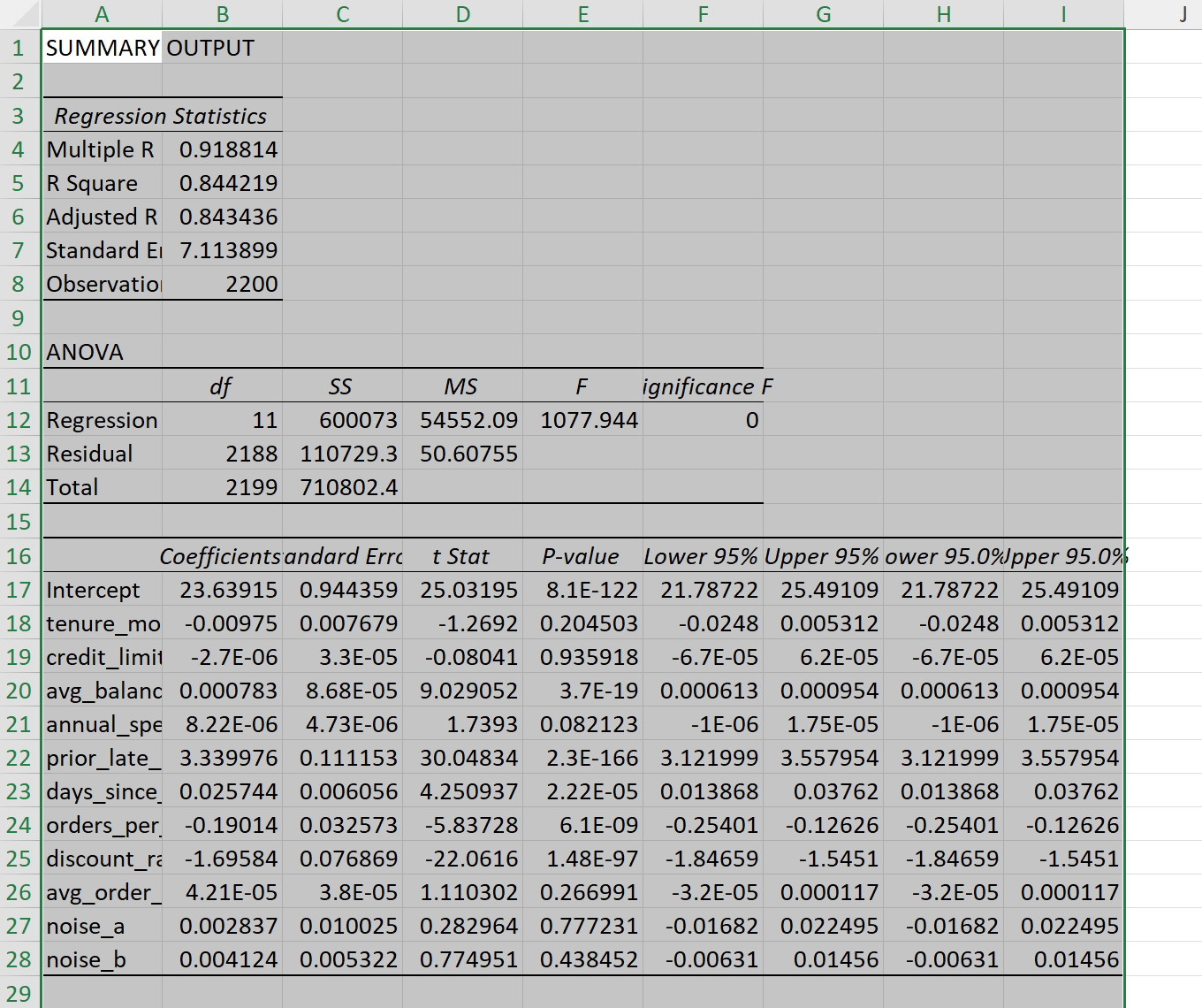
Here R Square is 0.844 and prior_late_count is +3.34, the same numbers as the Python fit. Notice the account-size columns (credit_limit, avg_balance, annual_spend) have small, shaky-looking coefficients. The next step shows why.
Check collinearity in Excel too
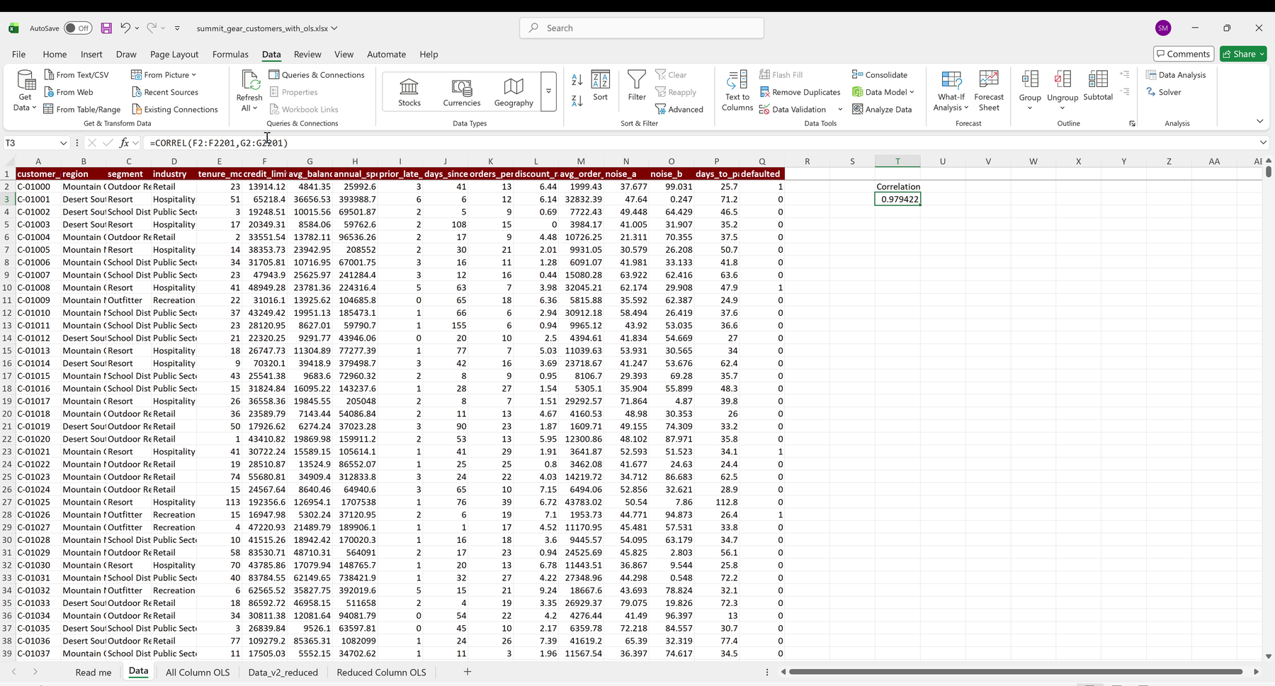
The Exercise 2 correlation matrix also runs here: Data Analysis -> Correlation, select the numeric predictor columns, and read the off-diagonal cells, the account-size cluster (credit_limit, avg_balance, annual_spend) sits near 1.0, the same signal you saw in Python.
Prune the redundant cluster and refit
Those three account-size columns are near-duplicates, so re-run the regression on only the predictors that carry distinct signal (avg_balance, prior_late_count, days_since_last_order, orders_per_year, discount_rate):
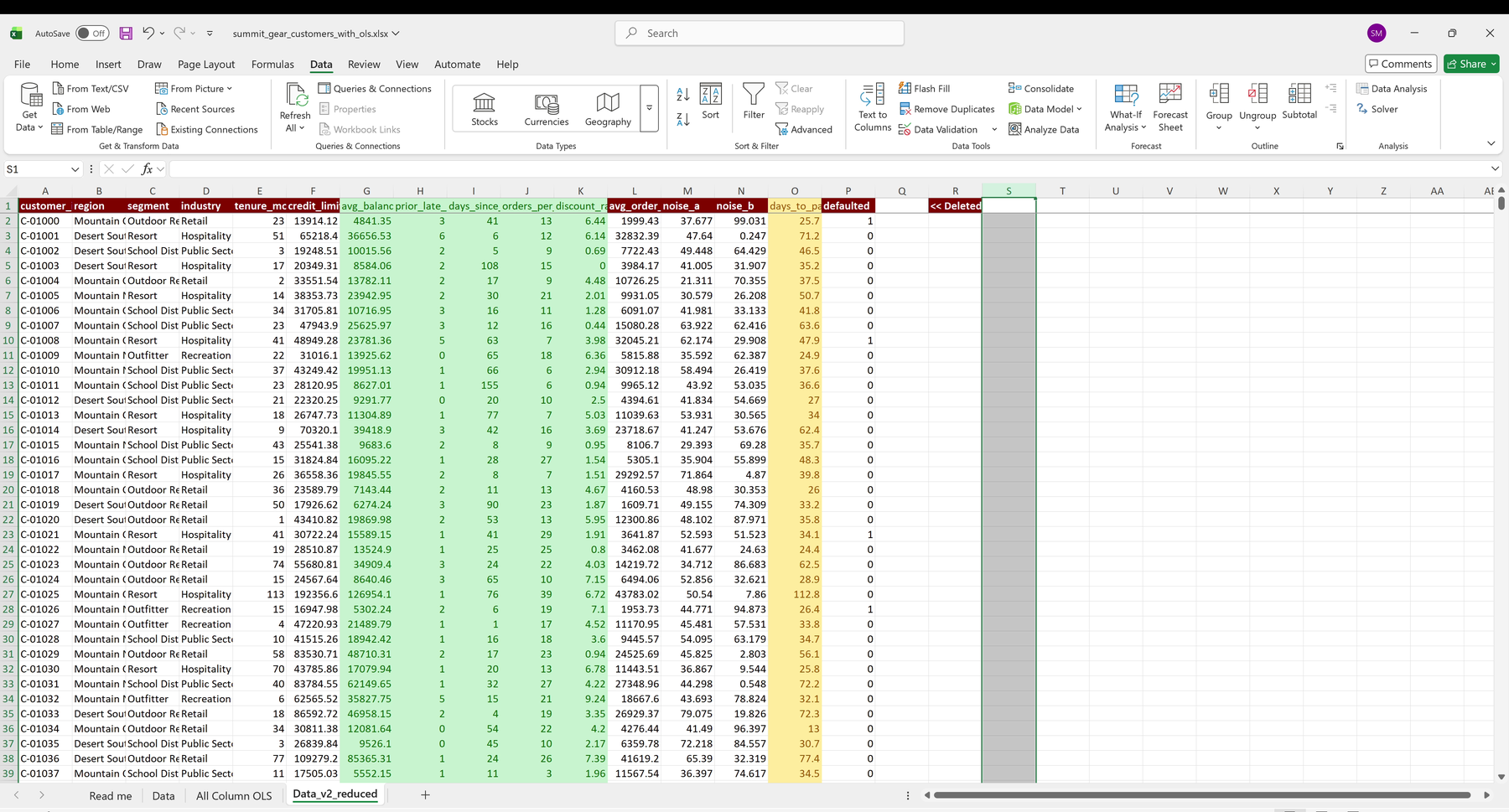
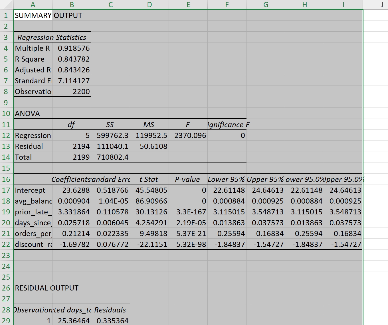
R² barely moves (still about 0.844), but the cluster's unstable coefficients are gone and avg_balance settles to a clean, readable value. That is the multicollinearity fix from Exercise 2, shown in Excel.
This is a genuinely fast way to get a first look at an OLS fit. It is an optional callback, not a parallel graded path, your graded work is the notebook.
Exercise 3, Fit logistic for defaulted, read odds and probabilities, pick a cutoff 25 pts
What to do here: fit a logistic model for defaulted, read the odds ratios and predicted probabilities in collections terms, and look at one cutoff.
The question changes shape. "Will this receivable go bad" is a yes/no, not a dollar amount, so OLS is the wrong tool, a linear model would predict probabilities below 0 and above 1. Logistic regression is built for a 0/1 outcome: it runs a linear score through a sigmoid that squashes any number into a probability between 0 and 1.
A short on-ramp (read this before you fit). Nothing before this week defined a probability or odds, so:
- A probability is a number from 0 to 1: the chance the outcome is 1.
- Odds are
p / (1 - p). A probability of 0.2 is odds of 0.25, or "1 to 4." - A logistic coefficient is read on the log-odds scale (the probability, odds, log-odds chain from lecture), which is awkward to read raw, so we report
exp(coef), the odds ratio: the multiplier on the odds of default per one-unit rise in that predictor, holding the others fixed. An odds ratio above 1 raises the odds of default; below 1 lowers them.
Specify. The target is defaulted. Choose a sensible predictor set, the clean payment-behavior predictors are the natural ones (prior_late_count, days_since_last_order, discount_rate, orders_per_year). Name your set and say in one line why each belongs and is known at decision time.
Let AI write the fit. Ask the tutor for the statsmodels logistic regression of defaulted on your predictors, printing the coefficient table, the odds ratios (exp(coef)), and the predicted probability for a couple of example customers. Run it, save the output.
statsmodels with sm.Logit(y, sm.add_constant(X)).fit() (or scikit-learn's LogisticRegression if you prefer), and use numpy for exp when you turn coefficients into odds ratios. Same install as Exercise 2: pip install pandas numpy statsmodels scikit-learn.Interpret (this is the graded part). Write a short paragraph that answers:
- Read the
prior_late_countodds ratio in plain words: each additional prior late payment multiplies the odds of default by about how much? - For one low-risk and one high-risk example customer, state the predicted probability the model gives, and say whether the ordering matches your business intuition.
- Note the base rate of default in the data (about 20%) and say why a model that outputs probabilities is more useful to a collections manager than a flat yes/no.
Pick a cutoff (and stop there). A probability is not yet a decision. To act on it you choose a cutoff: call everyone above it "predict default." Use 0.5 to start, and ask the AI for the one confusion matrix at that cutoff (true/false positives and negatives). Read it once and write one sentence: at a 0.5 cutoff, does the model catch most defaults or miss most of them? You will find it misses most, because defaults are only ~20% of the data, so 0.5 is a high bar. That is the whole point you carry into Week 9, choosing the right cutoff against the cost of a miss versus a false alarm is next week's job. Do not go past this one matrix.
Write the helper. Fill in sigmoid:
def sigmoid(z):
    """TODO: one sentence, what does this return?"""
    return None
What it takes and returns: sigmoid(z) takes a number z, the linear score, and returns a float probability between 0 and 1, computed as 1 / (1 + exp(-z)). Use math.exp or numpy.exp for the exponential. This is the function that turns a linear score into a probability, the engine of logistic regression, written once by hand. Quick sanity check: sigmoid(0) returns 0.5.
sigmoid is auto-checked with held-out inputs (for example sigmoid(0) == 0.5) and the fitted prior_late_count odds ratio is checked against the key (~1.87), so keep the signature and the docstring; the interpretation paragraph and the one-sentence cutoff read are read against the rubric. A final_check function at the end of the notebook runs several held-out checks across all three helpers (predicted_days, flag_collinear_pairs, sigmoid) and tells you, item by item, what is right and what is a little off, so run it and clear it before you submit.Exercise 4, Have an AI generate an HTML explainer, then assess it 25 pts
What to do here: once your three models are done, you complete the fourth graded piece, the explainer, entirely in the Lab 8 quiz.
The explainer is the judgment artifact of this lab, and it lives in the Lab 8 New Quiz, not on this page. After your models are done, the quiz walks you through it: it gives you the full prompt for generating a single self-contained HTML explainer with an external AI chat (Gemini, ChatGPT, or Claude), has you upload that lab_08_explainer.html, and then asks you to write your own assessment of whether it actually taught you anything. Generating a clean summary is what AI is good at; judging whether it is right and useful is your job, and that judgment is what earns the points.
Submit
Everything goes to the Lab 8 New Quiz, in the Week 8 module in Canvas. First finish your notebook, run every cell top to bottom so the fitted tables are saved, then File -> Download -> Download .ipynb. Then, in the quiz, submit three things:
- Upload your notebook (
.ipynb) with outputs saved, Exercises 1 to 3. - Generate and upload your explainer,
lab_08_explainer.html, using the prompt the quiz gives you. - Answer the assessment as the quiz's written question, in your own words.
You may resubmit as many times as you like; the latest attempt is kept. There is no time limit.
Rubric (100)
Four exercises, 25 points each. Exercises 1 to 3 each pair an auto-checked helper and a keyed number (read by the machine) with an interpretation read against the rubric. Exercise 4 is the uploaded AI-generated explainer plus your own-words assessment of it, both completed in the Lab 8 quiz. The read-against-the-rubric rows use the project-rubric anchors: full = correct and interpreted in collections terms with economic intuition; most = addresses it, interpretation thin; some = weak link to the question; little = missing or wrong. Award any whole-point value up to the maximum; reserve large drops for work substantively missing or wrong.
| # | Component | Pts | How scored |
|---|---|---|---|
| 1 | OLS fit + interpretation | 25 | predicted_days held-out + keyed R² (~0.84) (10, auto); two-coefficient + R² interpretation in collections terms (15, rubric) |
| 2 | Feature selection + collinearity | 25 | flag_collinear_pairs held-out + keyed reduced adj-R² (~0.843) (10, auto); the diagnose / keep-one / adjusted-R² justification (15, rubric) |
| 3 | Logistic fit + odds + cutoff | 25 | sigmoid held-out + keyed odds ratio (~1.87) (10, auto); odds-ratio + predicted-probability interpretation and the one-sentence 0.5-cutoff read (15, rubric) |
| 4 | AI-generated explainer + assessment | 25 | the uploaded HTML explainer covering the lab's three core ideas (10); your own-words assessment of it, answered as the Lab 8 quiz's written question (15); both rubric |
| Total | 100 |
A few reminders
- The helper signatures are a contract. The grader calls
predicted_days,flag_collinear_pairs, andsigmoidby name with held-out inputs. Do not rename them or change their parameters, or that auto-checked slice scores zero. The rest of your credit is untouched. - Save your outputs. Run every cell before you download so the fitted tables are in the
.ipynb. A notebook that does not run at all is flagged for the instructor to confirm as a zero, not silently failed. - AI writes the fits; you own the reading. Let an AI write every
statsmodels/sklearnline, and let an external AI chat build the explainer HTML in Exercise 4. The graded work is the interpretation, the feature-selection decision, the cutoff read, and your assessment of the explainer, and the on-page tutor will not write those before you have taken a pass. - An instructor assigns every judgment score. The interpretation, the verification, and your assessment of the explainer are read against the rubric by the instructor of record. An AI proposes; a person decides.
- A worked answer key is released after the deadline.
Summit Gear Co. is fictional. The dataset and the lab are custom-built for ACCTG 5150.